Final Evaluation

Hi, everyone!

This blog post contains a detailed review of the development of the Google Summer of Code project Module for Approximate Bayesian Computation. I will go over key points of the project and provide code snippets and links to commits that show the current state of the implementation. Along the way, I will point out different challenges encountered and future work to be done. Finally I will test the work product in a common example.

Project Abstract

Approximate Bayesian Computation (ABC) algorithms, also called likelihood free inference techniques, are a family of methods that can perform inference without the need to define a likelihood function (Lintusaari, 2016). Additionally, the ABC approach has proven to be successful over likelihood based methods for several models. We propose to implement a module for ABC in PyMC3, specifically Sequential Monte Carlo-ABC (SMC-ABC). Our work will signify a meaningful increase in the spectrum of models that PyMC3 will be able to run.

Main Objective

This project’s objective is to implement an ABC module in PyMC3 on the basis of the current implementation of the Sequential Monte-Carlo Algorithm.

Link to current PyMC3’s SMC code.

Link to a recent PR refactoring the SMC code.

What was done

• In this project a complete refactorization of the Sequential Monte Carlo code was made. Link to refactorized SMC-ABC code.
• We defined the SMC-ABC class with attributes that are particularly necessary for ABC. Link to SMC-ABC class code.
• A new PyMC3 distribution was added, the Simulator. Link to simulator.
• We defined a function to manage epsilon thresholds. Link to epsilon computation function.
• We defined a function to compute summary statistics. Link to summary statistics computation code.
• We defined functions to manage the different distance metrics available to the user. Link to distance metrics code.
• With the components metioned above, we defined a sampling function that applies a rejection kernel. Link to sampling function.

What is left to do

• This implementation would need several improvements in terms of performance. For example, parallelize the simulator function, which is the most expesive step in the sampler.
• In many cases the sampler encounters issues with covariance matrix computing and low or zero acceptance rates.

Links to core commits

These commits contain most of the new code.

• Refactor SMC ABC code.

• Add simulator distribution and distance functions.

• Refactor posterior and proposal distributions.

• Final changes to epsilon schedule computation.

Development process details

Now I will go over challenging points in the development process.

How do we define a PyMC3 model without a likelihood?

This was one of the first challenges we encountered. The conceptual basis of an ABC module is to provide the user with the API for perfoming inference on a model with no likelihood function.

ABC iteratevly compares the summary statistics computed from simulated data, with those of the observed data. Which presents the need for a variable inside the model that stores the observed data. This variable tipically is the likelihood.

In this SMC-ABC implemetation we constructed the Simulator distribution. This is a dummy distribution that only stores the observed data and a function to compute the simulated data.

Defining a Simulator distribution

This is a fraction of the simulator code:

class Simulator(NoDistribution):
	def __init__(self, function, *args, **kwargs):
        self.function = function
        observed = self.data

As you can see, this variable stores the Simulator function and the observed data. You can define it this way:

simulator = pm.Simulator('simulator', function, observed=data)

Link to simulator

How are Summary Statistics computed?

The user can choose between a predefined set of summary statistics. Also, the SMC-ABC sampler is able to perform inference using a combination of summary statistics, that is why the argument for this function is a list. The user can define it’s own summary statistic function and pass it to the sampler. Here is the function and use examples:

def get_sum_stats(data, sum_stat=['mean']):
    """
    Parameters:
    -----------
    data : array
        Observed or simulated data
    sum_stat : list
        List of summary statistics to be computed. 
        Accepted strings are mean, std, var. 
        Python functions can be passed in this argument.

    Returns:
    --------
    sum_stat_vector : array
        Array contaning the summary statistics.
    """
    if data.ndim == 1:
        data = data[:,np.newaxis]
    sum_stat_vector = np.zeros((len(sum_stat), data.shape[1]))

    for i, stat in enumerate(sum_stat):
        for j in range(sum_stat_vector.shape[1]):
            if stat == 'mean':
                sum_stat_vector[i, j] =  data[:,j].mean()
            elif stat == 'std':
                sum_stat_vector[i, j] =  data[:,j].std()
            elif stat == 'var':
                sum_stat_vector[i, j] =  data[:,j].var()
            else:
                sum_stat_vector[i, j] =  stat(data[:,j])

    return np.atleast_1d(np.squeeze(sum_stat_vector))

Default summary statistic is mean:

get_sum_stats(data)
array([-0.04784994])

Here we compute the mean, standard deviation and variance of a one dimensional array:

get_sum_stats(data, sum_stat=['mean', 'std', 'var'])
array([-0.04784994,  1.00437194,  1.008763  ])

Now I will define a custom summary statistic function and apply it on a two-dimensional array of data.

# custom summary statistic function
def custom_f(data):
    return np.square(data.mean()+data.var())

get_sum_stats(data.reshape(500,2), sum_stat=['mean', 'std', 'var', custom_f])
array([[-0.01314941, -0.08255046],
   [ 1.00339486,  1.00414964],
   [ 1.00680125,  1.0083165 ],
   [ 0.98734398,  0.85704276]])

In this dataframe is easier to observe how the summary statistics are displayed:

	feature1	feature2
mean	-0.013149	-0.082550
std	1.003395	1.004150
var	1.006801	1.008316
custom_f	0.987344	0.857043

This function is used internallly for the sampler for computing summary statistics.

Link to summary statistics computation code.

Distance metrics

Distance metrics are an argument of the SMC-ABC class. The user can choose any of the following distance metrics:

• Absolute difference.
• Sum of squared distance.
• Mean absolute error.
• Mean squared error.
• Euclidean distance.

Default option is absolute difference. Once the argument is read it is used in the rejection kernel.

Link to distance metrics code

Epsilon thresholds computation

An SMC-ABC sampler runs across a series of acceptance-rejection thresholds called epsilon. On this implementation the user can provide a sequence in the form of a list, otherwise they are computed taking a factor of the inter quantile range of the last simulated data.

Link to epsilon computation function.

Making all of these components work toghether

This is the sampler SMC-ABC function that combines the components above.

Examples

A trivial example

import pymc3 as pm
import numpy as np
import matplotlib.pyplot as plt

In this example I will try to estimate the mean and standard deviation of normal data. This problem could be solved using a likelihood, but is still good for testing the SMC-ABC sampler in a very basic instance.

# true mean and std
data.mean(), data.std()
(-0.04784993519517787, 1.004371943957994)

I defined a data simulator function that takes a mean and a scale parameter and return data of the same shape as the observed data.

def normal_sim(a, b):
    return np.random.normal(a, np.abs(b), 1000)

PyMC3 model:

with pm.Model() as example:
    a = pm.Normal('a', mu=0, sd=5)
    b = pm.HalfNormal('b', sd=1)
    s = pm.Simulator('s', normal_sim, observed=data)
    trace_example = pm.sample(step=pm.SMC_ABC())

Using absolute difference as distance metric
Using ['mean'] as summary statistic
Sample initial stage: ...
Sampling stage 0 with Epsilon 1.915432
100%|██████████| 500/500 [00:00<00:00, 836.37it/s]
Sampling stage 1 with Epsilon 0.939661
100%|██████████| 500/500 [00:00<00:00, 717.28it/s] 
Sampling stage 2 with Epsilon 0.452645
100%|██████████| 500/500 [00:00<00:00, 710.28it/s]

pm.summary(trace_example)

	mean	sd	mc_error	hpd_2.5	hpd_97.5
a	-0.091348	0.236713	0.009575	-0.449605	0.370533
b	1.161391	1.935439	0.080310	0.028291	3.522031

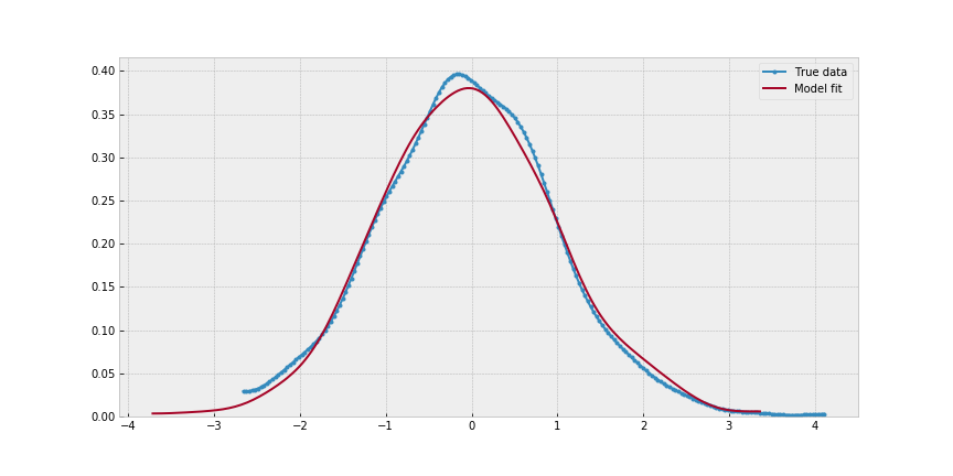
_, ax = plt.subplots(figsize=(12,6))
pm.kdeplot(data, label='True data', ax=ax, marker='.')
pm.kdeplot(normal_sim(trace_example['a'].mean(), 
		      trace_example['b'].mean()), ax=ax)
ax.legend();

Lotka–Volterra

In this example we will try to find parameters for the Lotka-Volterra equations. A common biological competition model for describing how the number of individuals of each species changes when there is a predator/prey interaction (A Biologist’s Guide to Mathematical Modeling in Ecology and Evolution,Otto and Day, 2007). For example, rabbits and foxes. Given an initial population number for each species, the integration of this ordinary differential equations (ODE) describe curves for the progression of both populations. This ODE’s take four parameters:

• a is the natural growing rate of rabbits, when there’s no fox.
• b is the natural dying rate of rabbits, due to predation.
• c is the natural dying rate of fox, when there’s no rabbit.
• d is the factor describing how many caught rabbits let create a new fox.

This example is based on the Scipy Lokta-Volterra Tutorial.

from scipy.integrate import odeint

First we will generate data using known parameters.

# Definition of parameters
a = 1.
b = 0.1
c = 1.5
d = 0.75

# initial population
X0 = [10., 5.]
# size of data
size = 1000
# time lapse
time = 15
t = np.linspace(0, time, size)

# ODEs
def dX_dt(X, t, a, b, c, d):
    """ Return the growth rate of fox and rabbit populations. """

    return np.array([ a*X[0] -   b*X[0]*X[1] , 
                  -c*X[1] + d*b*X[0]*X[1] ])

With this function I will generate noisy data to be used as observed data.

def add_noise(a, b, c, d):
    noise = np.random.normal(size=(size, 2))
    simulated = simulate(a, b, c, d)
    simulated += noise
    indexes = np.sort(np.random.randint(low=0, high=size, size=size))
    return simulated[indexes]

Then I define the simulator function, which performs the integration of the ODE.

def simulate(a, b, c, d): 
    return odeint(dX_dt, y0=X0, t=t, rtol=0.1, args=(a, b, c, d))

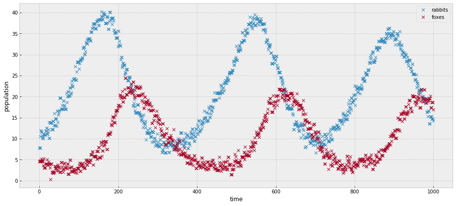
# plotting observed data.
observed = add_noise(a, b, c, d )
_, ax = plt.subplots(figsize=(16,7))
ax.plot(observed, 'x')
ax.set_xlabel('time')
ax.set_ylabel('population');

# PyMC3 model using Half-normal priors for each parameter, 
# given that none of them can take negative values.
with pm.Model() as model:
    a = pm.HalfNormal('a', 1, transform=None)
    b = pm.HalfNormal('b', 0.5, transform=None)
    c = pm.HalfNormal('c', 1.5, transform=None)
    d = pm.HalfNormal('d', 1, transform=None)
    simulator = pm.Simulator('simulator', simulate, observed=observed)
    trace = pm.sample(step=pm.SMC_ABC(n_steps=50, min_epsilon=70, iqr_scale=3), 
                      draws=500)

Using absolute difference as distance metric
Using ['mean'] as summary statistic
Sample initial stage: ...
Sampling stage 0 with Epsilon 8.542185
 92%|█████████▏| 458/500 [00:09<00:00, 46.22it/s]
  warnings.warn(warning_msg, ODEintWarning)
100%|██████████| 500/500 [00:10<00:00, 47.18it/s]

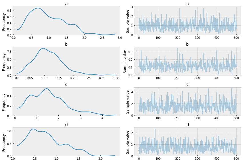
pm.traceplot(trace);

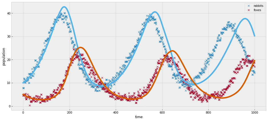
_, ax = plt.subplots(figsize=(16,7))
ax.plot(observed, 'x')
ax.plot(simulate(trace['a'].mean(), trace['b'].mean(), 
                 trace['c'].mean(), trace['d'].mean()))
ax.set_xlabel('time')
ax.set_ylabel('population');

pm.summary(trace)

	mean	sd	mc_error	hpd_2.5	hpd_97.5
a	0.885993	0.302209	0.013313	0.433645	1.471938
b	0.082683	0.030849	0.001362	0.039713	0.140521
c	1.529694	0.709558	0.033590	0.458533	2.923218
d	0.874219	0.323623	0.015791	0.487962	1.729934

Future Work

The results we have observed so far are a good start but this module is still in an experimental phase. As I mentioned above, this sampler could be faster if some performance issues were adressed. Mainly, the cost of the simulator function, that is called in every iteration of the sampler and can add up to significant amounts.

On the other hand, this implementation is quite unstable, meaning that some runs can show reasonably good results and others can present problems with covariance matrix computation or low acceptance rates. Which results in poor parameter estimation. In future work, we would like to include tunning of the number of acceptance/rejection steps that each chain goes through. This might deal efectively with the low acceptance rate issues. Besides, this SMC-ABC implementation cannot sample from transformed PyMC3 variables, as it encounters boundary issues.

As you can see there is still quite a bit to polish and improve on, which is why this project’s work will extend after the Google Summer of Code program is over.

Thanks to Google Summer of Code for promoting open-source projects and bringing developers and students closer to open-source communities.