Integrating SMC-ABC step method into PyMC3
Hello everyone! :)
We are approaching the second evaluation period in GSoC 2018 and the Sequential Monte Carlo ABC step method is slowly but surely coming into place.
%matplotlib inline
import numpy as np
import pymc3 as pm
Here I am showing how it can sample from a normal distribution using a set of predefined epsilon thresholds, or computing them by scaling the interquartile range with the iqr_scale parameter. It will continue to sample until a minimum epsilon value is reached.
# true data
data = np.random.normal(0, 5, 1000)
# ladder of pre-defined epsilons
epsilon = np.linspace(1, 0.5, 8)
# parameters for the step method
step_kwargs = {'minimum_eps':0.55, 'iqr_scale': 2}
Notice that in this model there is no likelihood, only a prior for the mean.
with pm.Model() as model:
    a = pm.Normal('a', mu=0.5, sd=1)
    trace = pm.sample(step=pm.SMC_ABC(observed=data), step_kwargs=step_kwargs)
In future implementations the choice of summary statistics and distance function will be available to the user. As for now they are hidden and hardcoded.
UserWarning: Warning: SMC is an experimental step method, and not yet recommended for use in PyMC3!
  warnings.warn(EXPERIMENTAL_WARNING)
Init new trace!
Sample initial stage: ...
Epsilon: 0.7574 Stage: 0
Initializing chain traces ...
Sampling ...
100%|██████████| 100/100 [00:00<00:00, 2460.48it/s]
Epsilon: 0.7574 Stage: 1
Initializing chain traces ...
Sampling ...
100%|██████████| 100/100 [00:03<00:00, 30.31it/s]
Epsilon 0.3324 < minimum epsilon 0.5000
Sample final stage
Initializing chain traces ...
Sampling ...
100%|██████████| 500/500 [00:17<00:00, 29.23it/s]
pm.traceplot(trace);
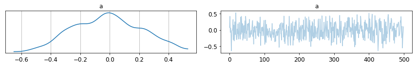
pm.summary(trace)
| mean | sd | mc_error | hpd_2.5 | hpd_97.5 | |
|---|---|---|---|---|---|
| a | -0.02 | 0.23 | 0.01 | -0.43 | 0.44 |
Results are not quite perfect yet, but they are looking good so far. How to provide a simulator/emulator environment with PyMC3 is one of the main challenges left.
Here is a link to my SMC-ABC branch, in case you want to take a look at the source code :)