Last friday I participated in PyMC3’s journal club meeting. I talked to PyMC3 members about my Google Summer of Code project. In this post I am showing the jupyter notebook I used to guide the talk. It was very helpful to get feedback from the developers about my project ideas. I look forward to join in next journal club meetings :).

Google Summer of Code project

Developping a module for Approximate Bayesian Computation for PyMC3

Student: Agustina Arroyuelo

Mentors: Junpeng Lao, Osvaldo Martin

%matplotlib inline
import numpy as np
import pymc3 as pm
import matplotlib.pyplot as plt
import arviz as az
plt.style.use('bmh')

What is ABC?

Approximate bayesian computation is a class of computational methods, also called Likelihood free inference methods, that bypass the evaluation of the likelihood function.(Sunnaker, 2013).

Why do we need Approximate Bayesian Computation or Likelihood Free Inference?

We need ABC because for some models the likelihood function is very complex and it’s evaluation can be computationally costly. These models are typically called simulator based model. ABC is key in parameterizing simulator based models.

What are Simulator Based Models? $M(\theta, V) = y$

The likelihood function cannot be computed or is intractable due to their stochastic nature
Typically have multiple parameters
Given a set of parameters, it is ‘easy’ to generate data from them

The most simple ABC algorithm is rejection ABC

# rejection ABC sampling
def rejection_abc(model=None, samples=1000, ϵ=0.5, plot=True):
    """
    Rejection ABC sampling 
    
    Parameters
    ----------
    model: pymc3 model
    samples : int
      Number of sampling steps
    ϵ : int or float
      Threshold value
      
    Returns
    -------
    accepted : list
      List of accepted θ
    """    
    
    model = pm.modelcontext(model)
    prior = model.unobserved_RVs[0]
    data = model.observed_RVs[0].observations
    size = len(data) 
    scale = data.std()
    mean = data.mean()
    accepted = []
    ys = []
    
    for _ in range(samples): 
        θ = prior.random() # prior sample
        y_θ = np.random.normal(loc=θ, scale=scale, size=size) # simulator
        ys.append(y_θ)
        if np.absolute(mean - y_θ.mean()) < ϵ: # distance function, summary statistic
            accepted.append(θ)
    
    if plot:
        _, ax = plt.subplots(1, 2, figsize=(12, 4))
        az.kdeplot(data, label='data', ax=ax[0])
        az.kdeplot(accepted, label='posterior', c='C7', ax=ax[1])
        [ax[i].scatter(accepted, [0]*len(accepted), marker='|', label='θ', c='C4') for i in range(len(ax))]
        [ax[i].legend() for i in range(len(ax))]
        [ax[i].set_yticks([]) for i in range(len(ax))]

    return accepted, ys

data = np.random.randn(1000)
with pm.Model() as model:
    a = pm.Normal('a')
    l = pm.Normal('l', observed=data)

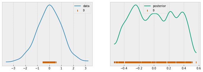
rej_abc = rejection_abc(model=model)

png

For likelihood free inference we need…

A simulator based model
To choose a Summary statistic or a vector of them
A threshold
A distance function

SMC - ABC is a bit more complex…

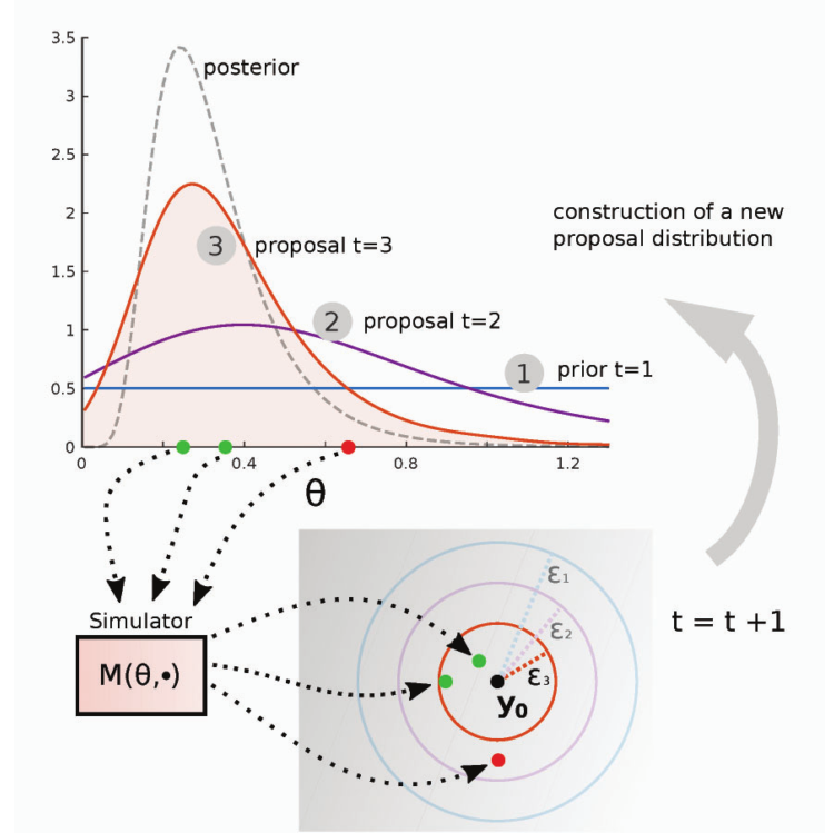
png (Lintusaari, 2016)

1- $\theta$’s are drawn from the prior, if it is the first stage, or proposal distribution if it is not.

2- They are passed to the simulator model.

3- The output $y$ from the simulator are compared with the true data $y_0$ using a distance $d$ function and a threshold $\epsilon$.

4- The accepted parameters are weighted accoding to $w^{(i)} \alpha \frac{p(\theta^{(i)})}{\phi(\theta^{(i)})}$ with $\phi$ being the proposal distribution.

The weight of $\theta$ is proportional to the density of $\theta$ in the prior over the density of $\theta$ in the proposal distribution

5- Return to 1-, $\epsilon$ decreases.

Towards the implementation of an ABC module in PyMC3…

Conceptually SMC-ABC is similar to the current implementation of SMC were every step is a rejection ABC instead of MCMC.
Simulator will be a variable inside a PyMC3 model, similar to pm.Deterministic variable, that takes parameters $\theta$, a distance function and a function that simulates data.
Simulator objects will tell the sampler if the parameters were accepted or not accepted.

pm.Simulator('name', function=F(), distance='weighted Euclidean', observed=data, epsilon=5, params=[α, β, γ], sum_stat='')

Thresholds are typically determined by simulating a pool of $(y, \theta)$ pairs and setting $\epsilon$ in a quantile of this distribution, for example 1%.

(Beaumont, 2002)

# ys is a pool of simulated data
_, ys = rejection_abc(model=model, samples=50000, plot=False)

from scipy.stats.mstats import mquantiles
threshold = mquantiles(ys, prob=[0.99])[0]

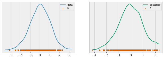
reject_abc, ys = rejection_abc(model=model, samples=500, ϵ=threshold)

png

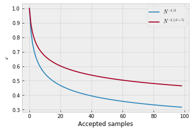
Thresholds usually decrease like $N^{-1/4}$ or $N^{-1/(d+5)}$ where d is the dimension of the parameter space and N the number of accepted samples.

plt.plot([i**(-1/4) for i in range(1,100)], label='$N^{-1/4}$')
plt.plot([i**(-1/(1+5)) for i in range(1,100)], label='$N^{-1/(d+5)}$') # for one-dimensional data
plt.xlabel('Accepted samples')
plt.ylabel('$ϵ$')
plt.legend(); 

Weights

$w^{(i)} \alpha \frac{p(\theta^{(i)})}{\phi(\theta^{(i)})}$

Distance functions

The user should be able to choose from a set of distance functions. Interesting blog post about distance metrics

Summary statistics

Curse of dimensionality
Local informative summary statistics and global ones, are different.

ABC (R package), PyABC

Ending remarks

In this Google Summer of Code project we will use and refactor the current implementation of SMC, to add the necessary components for an SMC-ABC module.
We will include a new variable for PyMC models, called simulator. It will store the sequence of thresholds and distance functions, and comunicate the accepted parameters
We are going to explore different methods for the choices of thresholds, distances and summary statistics, trying to base our decissions in existing implementations.

PyMC3's Journal Club